Put a Hex on it: Introducing new Uber H3 Capabilities

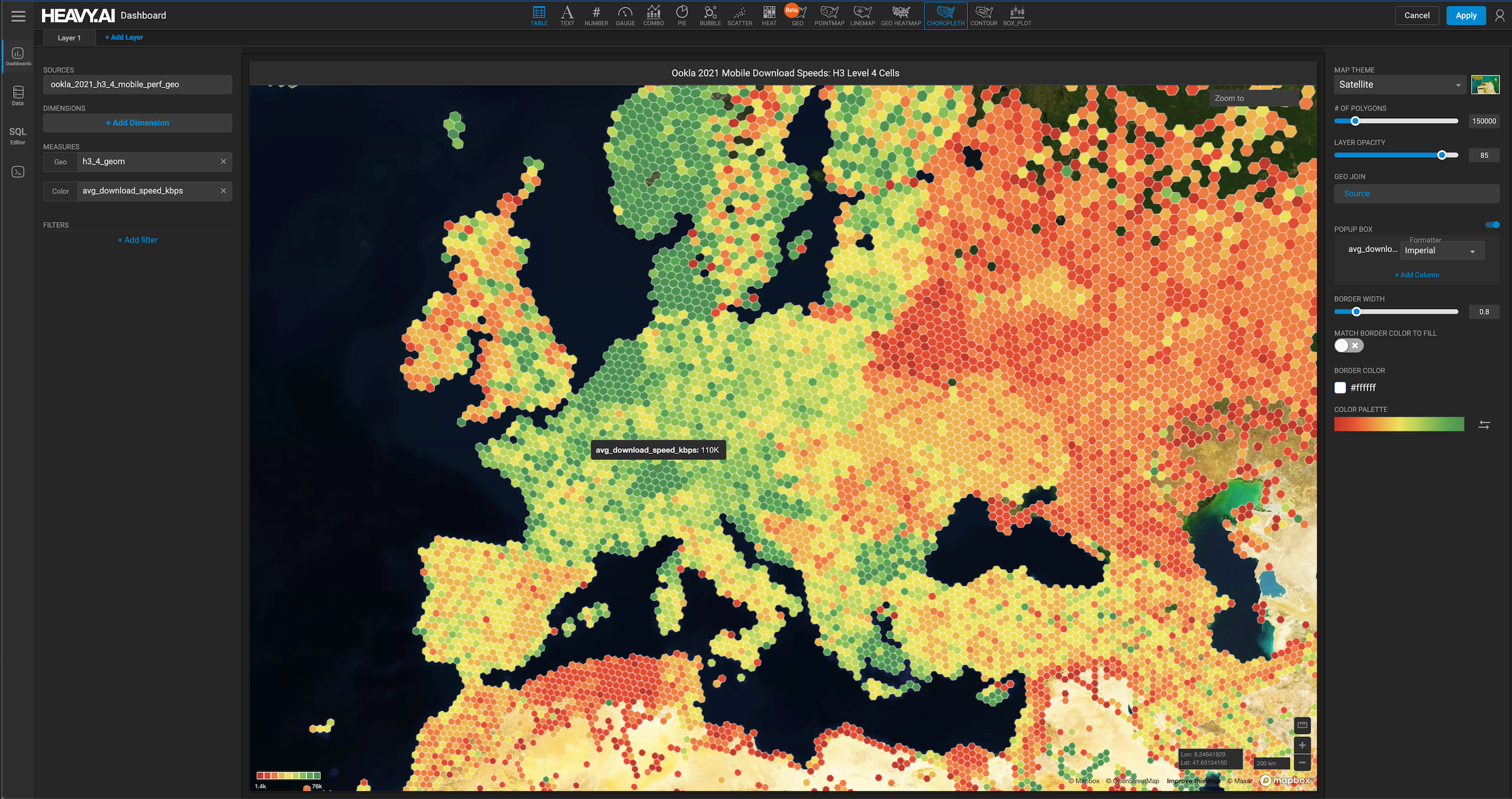
With HEAVY.AI’s GPU-accelerated analytics platform, analysts can easily visualize and interrogate massive datasets interactively and in real-time. The platform is particularly useful for analysis and visualization of large-scale geospatial data, as it can both render large geospatial data sources with the built-in GPU-powered HeavyRender engine while powering deeper analysis via GPU-accelerated geospatial SQL and joins, based on the Open Geospatial Consortium (OGC) standard. Now, as part of our 8.4 release, we are adding extensive new capabilities to use Uber’s H3 Indexing functionality to allow new forms of spatial analysis.

‍

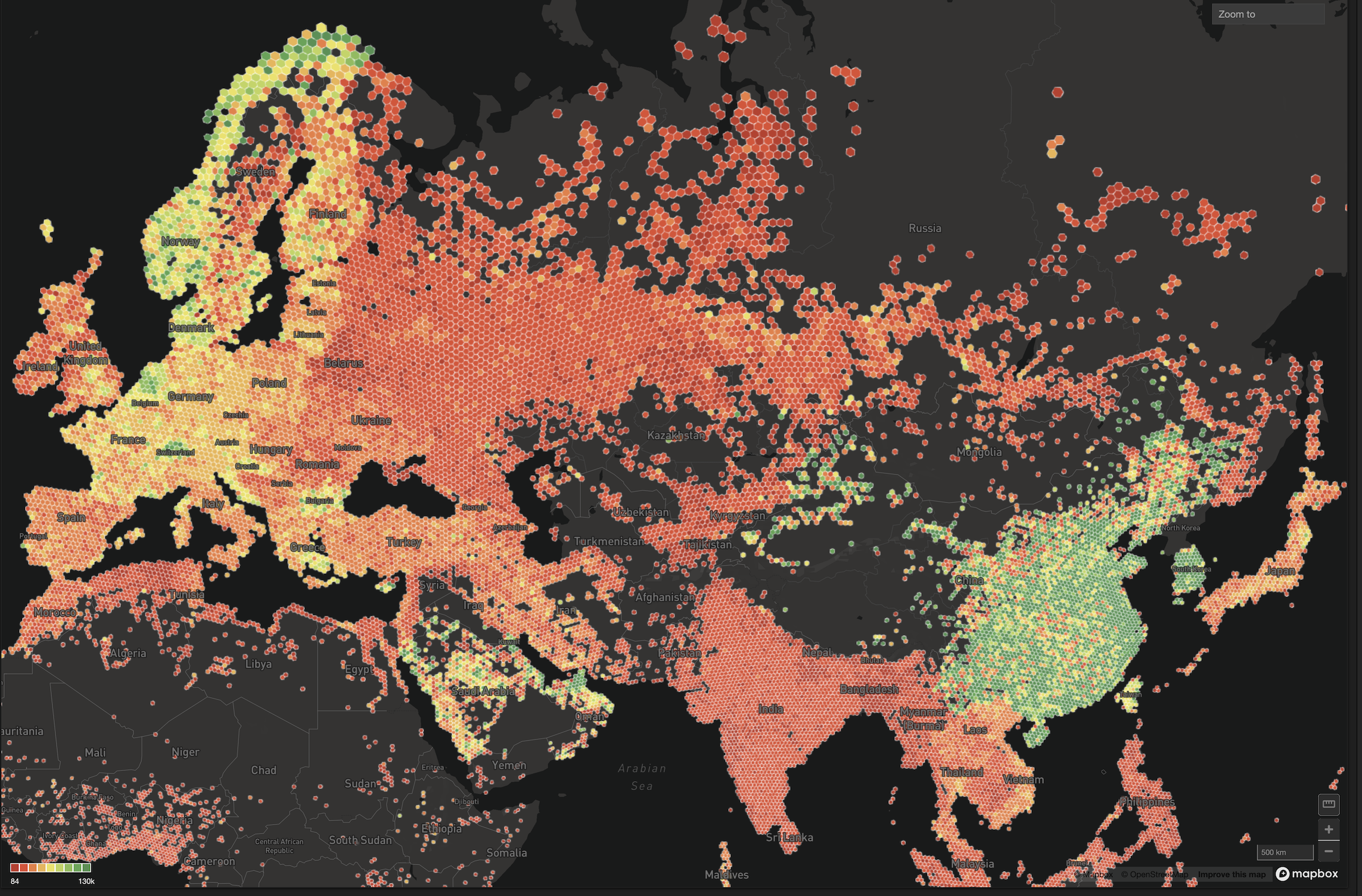
H3 offers a transformative value proposition for data analytics by providing a highly efficient and scalable geospatial indexing system. Its hexagonal grid structure minimizes quantization errors and ensures uniform coverage of spatial data, making it ideal for analyzing large, complex datasets within the HEAVY.AI platform. Unlike traditional square or administrative grid systems, H3's hierarchical design enables seamless aggregation and disaggregation of data at multiple resolutions, empowering analysts to explore patterns at varying levels of granularity. This flexibility is critical for partners dealing with massive spatio-temporal data, such as transportation, urban planning, and logistics, where understanding localized trends can drive actionable insights. Link

‍

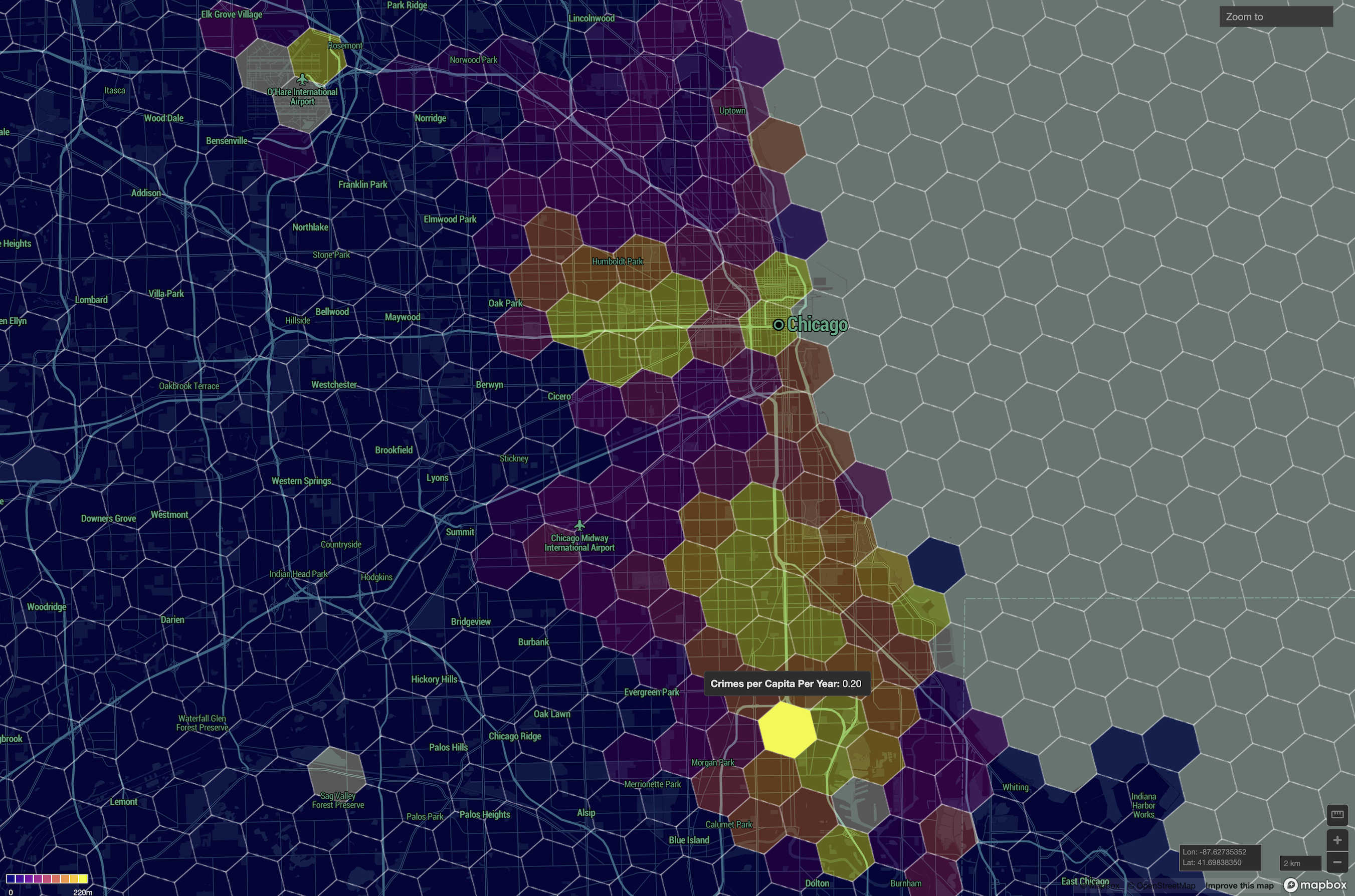
Another key advantage of H3 lies in its ability to simplify spatial joins and enable high-performance geospatial analytics. By encoding geographic locations into unique cell IDs, H3 eliminates the need for computationally expensive spatial predicates during data integration. This makes it an invaluable tool for combining disparate datasets, as it provides a more complete picture when trying to understand mobility patterns, environmental factors, or customer behavior.  Additionally, the system's compatibility with machine learning workflows allows organizations to build predictive models that leverage spatial features, such as risk assessment or demand forecasting. Whether it's visualizing city cores, optimizing delivery routes, or identifying high-demand zones in retail and transportation, H3 empowers businesses to derive actionable insights from their geospatial data with unparalleled precision and efficiency

‍

‍

The Specifics: 

‍

H3 is a global indexing system based on a multi-resolution hexagonal grid, developed at Uber. This allows world-space coordinates to be indexed to a unique 64-bit integer value which classifies that location by its closest surrounding hexagonal (or pentagonal) cell at resolutions down to approximately 0.5m accuracy. Each resolution step results in around a 3x drop in precision, with the coarsest representation having an accuracy of around 1200km. The cell indices can be used as a lightweight spatial coordinate representation, and also as join keys for spatial analysis operations. Any cell index can trivially be reduced in accuracy by simply masking off the lower-order bits of the value, which allows for various methods of optimizing the join operation.

‍

HeavyDB has included a simple H3 implementation since v6.0, but it was based on an older and now deprecated version of the H3 SDK. For v8.4 we deprecated the original implementation and introduced a completely new one based on the latest v4.2.0 H3 SDK. As before, the H3 operations are exposed as Extension Functions which can be called from SQL. Many of the functions mirror the previous implementation, but there are new additions, and more will be added in upcoming HeavyDB releases.

‍

Example Use Case: Erosion Modeling

‍

Perhaps the most common use of H3 encoding is in joining raster datasets at a common resolution.  For example, consider erosion modeling.  Modeling of erosion requires considering the slope of terrain and its land cover. Flat terrain with forest cover intercepts rain and minimizes erosion, whereas slope bare terrain is inherently erosion prone.  

‍

We can easily get both terrain slope and landcover from the US National Map. However the National Elevation Dataset is typically available at 10m resolution whereas Landcover is available only at 30m. How can we efficiently join such data?

‍

If we import both datasets using HEAVY.AI defaults, they will automatically be converted to WGS84 longitude and latitude with attributes raster_lon and raster_lat.  Our lowest resolution data is 30m, so avoiding interpolation for the moment, let's use H3 Level 8 hexagons.  Based on the provided resolution tables, this is the highest resolution hex grid above 30m. We don’t want to use anything lower simply to avoid gaps between our hexagons.  

‍

Here is the SQL we’ll use to make an integrated erosion prediction table with these two factors:

‍

Create table erosion as 

Select

   Avg(terrain.slope) as avgSlope,

   Approx_percentile(terrain.slope, 0.90) as p90slope, 

   Approx_median(landcover.cover_type) as median_landcover_type, 

  St_setsrid(St_point(terrain.raster_lon, terrain.raster_lat),4326) as geom 

From 

Terrain, Landcover 

Where 

H3_LonLatToCell(terrain.raster_lon, terrain.raster_lat, 8) = 

H3_LonLatToCell(landcover.raster_lon, landcover.raster_lat, 8)

Group by 

H3_LonLatToCell(terrain.raster_lon, terrain.raster_lat, 8)

‍

The resulting table has one row per hexagon, with a set of measures characterizing both layers in that hexagon. For continuous measures like slope, you can use any of the many aggregators available on the platform. APPROX_PERCENTILE for example is useful in quickly characterizing extreme slopes in a cell, which for erosion purposes provide an estimated range. For categorical measures, the median characterizes cell land cover in this case based on dominant type.  

‍

While this example is very specific this same query pattern holds across many use cases. You as the user need to make two fundamental decisions: which spatial scale is appropriate given the phenomenon of interest and available compute, and which aggregation metrics are most appropriate.  

‍

How to expand the use case

‍

A variety of related use cases can also follow on the above. For example, if you had measured erosion rates from field data, you could also H3 Hex encode those sample points and add measured_erosion as the first column to the table above. This table structure can then be used in any predictive modeling tool in HEAVY.AI. You can, for example, use Random Forest Regression trained on 80% of your rows with observations, test against a withheld 20%, then inference across a large landscape including many sites with no field measurements.  

‍

Summary

‍

In summary, H3 allows you to set up a sampling framework based on nearly equal sized units, and without fusing with spatial bounds and dataset alignments. You can use this directly for machine learning as above, or with some filtering to avoid spatial auto-correlation can pass to statistical tools. 

‍

Last but not least, you can render any of the integrated cell values or categories.  This currently (as of HeavyDB v8.4) requires that you CTAS the table to render the polygons, but additional functions to directly output live geometry will be added in a future release. 

‍

HEAVY.AI Uber H3 Functions

‍

The functions available in this initial new release are as follows:

‍

Coordinates to H3 Indices

‍

H3_PointToCell(POINT p, INTEGER resolution) -> BIGINT

H3_LonLatToCell(DOUBLE lon, DOUBLE lat, INTEGER resolution) -> BIGINT

‍

These functions take a world-space coordinate (in WGS84/SRID4326) as either POINT or DOUBLE, and a resolution value as INTEGER (which must be in the range 0 to 15) and return an H3 index as a BIGINT corresponding to the cell at that resolution with a center point nearest to the given point.

‍

H3 Indices to Coordinates

‍

H3_CellToLon(BIGINT cell) -> DOUBLE

H3_CellToLat(BIGINT cell) -> DOUBLE

‍

These functions take an H3 Index value as BIGINT and convert it back to a world-space coordinate (in WGS84/SRID4326) returning the longitude or the latitude value respectively of the center point of the cell represented by the input index.

‍

Conversions to and from Hex String Representation

‍

H3_CellToString_TEXT(BIGINT cell) -> TEXT ENCODING DICT

H3_CellToString_TEXT_NONE(BIGINT cell) -> TEXT ENCODING NONE

‍

These functions take an H3 Index value as BIGINT and convert it to the corresponding H3 Hex String representation. There are two variants of the function depending on whether the output needs to be a Dictionary-Encoded or None-Encoded TEXT value.

‍

H3_StringToCell([TEXT ENCODING DICT|TEXT ENCODING NONE]) -> BIGINT

‍

This function performs the reverse, taking a H3 Hex String as either a Dictionary-Encoded or None-Encoding TEXT value, and returning the corresponding numeric representation as BIGINT.

‍

Getting the Index Parent

‍

H3_CellToParent(BIGINT cell, INTEGER resolution) -> BIGINT

‍

This function takes an H3 Index value as BIGINT and returns the H3 Index value of the parent cell containing the input cell, at the specified resolution (larger).

‍

Checking Index Validity

‍

H3_IsValidCell(BIGINT cell) -> BOOL

‍

This function checks an H3 Index value for validity.

‍

Converting Index to Geometry

‍

H3_CellToBoundary_WKT(BIGINT cell) -> TEXT ENCODING DICT

‍

This function takes an H3 Index as BIGINT and returns a WKT (Well-Known Text) representation of the geo POLYGON of the cell boundary as a Dictionary-Encoded TEXT value.

‍

Example Renders

‍

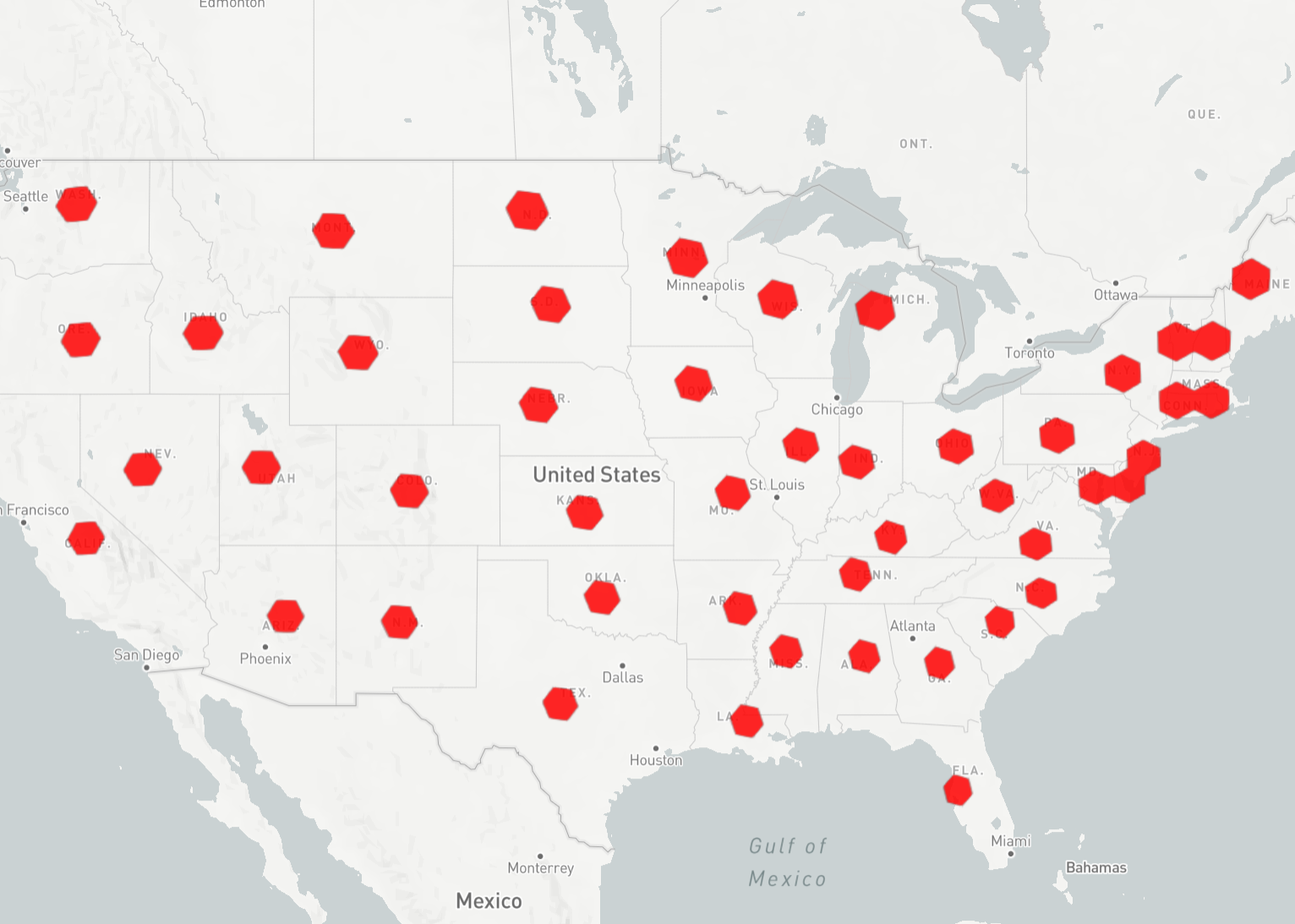
Here is a simple render of the hex POLYGONs generated by the following query, of the H3 cells at Resolution 3 that contain the centroid points of each US state boundary polygon, 

‍

SELECT H3_CellToBoundary_POLYGON(H3_LonLatToCell(ST_X(ST_Centroid(geom)), ST_Y(ST_Centroid(geom)), 3)) FROM heavyai_us_states

‍

‍

Future Development

‍

Future releases will include more functionality, such as:

• Converting H3 Indices to POLYGON Geometry (hexagon or pentagon) for rendering or more accurate spatial comparisons using the existing ST function set.

• Converting an H3 Index to a POINT type rather than separate scalar longitude/latitude

• Converting other geometry types (e.g. linestrings or polygons) to a list of Index values representing the nominally contiguous region of cells containing the given geometry.

‍

‍

‍